![Ω = 2.00π rad/sample; in (−π, π] it is 0 rad/sample. Wheel: the unit circle with marks n = 0 to 7 at angle Ωn, an arrow from the centre to mark 1 and an arc for Ω; marks 0, 1, 2, 3, 4, 5, 6 and 7 sit on one spot. Stems x[n] = cos(Ωn) for n = 0 to 15, starting 1, 1, 1, 1, 1, 1, 1, 1.](/thumbs/discrete-frequency-dark.webp)
![Ω = 2.00π rad/sample; in (−π, π] it is 0 rad/sample. Wheel: the unit circle with marks n = 0 to 7 at angle Ωn, an arrow from the centre to mark 1 and an arc for Ω; marks 0, 1, 2, 3, 4, 5, 6 and 7 sit on one spot. Stems x[n] = cos(Ωn) for n = 0 to 15, starting 1, 1, 1, 1, 1, 1, 1, 1.](/thumbs/discrete-frequency-light.webp)
Lesson 1★ Essential15 minYou are hereRead
Frequency in discrete time
See digital frequency as a turn per sample, why the frequency axis closes into a circle, and how to convert among its four common scales.
Chapter 12
Four lessons in Part V, Discrete-time Fourier analysis. Read them in order, or start anywhere: a prerequisite is a link, never a gate.
Start with 12.1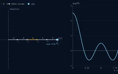
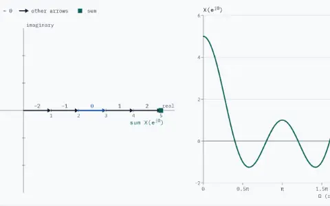
![Size of the spectrum of 0.8ⁿu[n] multiplied by e^{jΩ₁n}, for Ω₁ = 1.00π rad/sample. Solid curve, after the shift: peaks of height 5 at both ends, −π and π, which are the same point. Dashed curve, x alone: a peak of height 5 at 0 rad/sample.](/thumbs/dtft-properties-dark.webp)
![Size of the spectrum of 0.8ⁿu[n] multiplied by e^{jΩ₁n}, for Ω₁ = 1.00π rad/sample. Solid curve, after the shift: peaks of height 5 at both ends, −π and π, which are the same point. Dashed curve, x alone: a peak of height 5 at 0 rad/sample.](/thumbs/dtft-properties-light.webp)
![Stems of the test sine x[n] (dots) and the output y[n] (squares) at Ω = π, samples 0 to 23. 4 tests stamped on the gain and phase panels: 0.25π, gain 0.679, phase −28.7°; 0.5π, gain 0.447, phase −26.6°; 0.75π, gain 0.357, phase −14.6°; π, gain 0.333, phase 0.0°. A thin curve, from the equation, runs through them.](/thumbs/dt-frequency-response-dark.webp)
![Stems of the test sine x[n] (dots) and the output y[n] (squares) at Ω = π, samples 0 to 23. 4 tests stamped on the gain and phase panels: 0.25π, gain 0.679, phase −28.7°; 0.5π, gain 0.447, phase −26.6°; 0.75π, gain 0.357, phase −14.6°; π, gain 0.333, phase 0.0°. A thin curve, from the equation, runs through them.](/thumbs/dt-frequency-response-light.webp)
After this chapter
The chapters either side, and the rest of Part V in the library.