Skip to content

Chapter 15

Spectral analysis in practice

Six lessons in Part V, Discrete-time Fourier analysis. Read them in order, or start anywhere: a prerequisite is a link, never a gate.

Start with 15.1
0 of 6 read5 on the essential pathabout 128 minutes

Lessons in this chapter

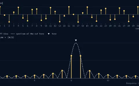
Top: 32 samples of a cosine at k₁ = 8.50 bins, as stems from sample 0 to 31. Bottom: the DFT as bars at bins 0 to 16, sizes ÷ (N/2), on the dashed spectrum of the cut tone; a triangle marks the tone at 8.50 bins. Tallest bar 8 at 0.6407; bar 7 0.2183, bar 9 0.6346; bar 16 0.0625. 59.0 % of the energy is outside the peak bar.Top: 32 samples of a cosine at k₁ = 8.50 bins, as stems from sample 0 to 31. Bottom: the DFT as bars at bins 0 to 16, sizes ÷ (N/2), on the dashed spectrum of the cut tone; a triangle marks the tone at 8.50 bins. Tallest bar 8 at 0.6407; bar 7 0.2183, bar 9 0.6346; bar 16 0.0625. 59.0 % of the energy is outside the peak bar.

Lesson 1 Essential20 minYou are hereRead

Windowing & spectral leakage

See why a tone between bins spreads into every bin, then taper the record's ends so a weak tone beside a strong one stands out.

The flat-top window. Shape panel: w[n] against n/N from 0 to 1. Spectrum panel: |W| in dB relative to its peak, against the offset from the tone, 0 to 16 bins. Main lobe 10.0 bins; the bracket marks half of it, from 0 to the first zero at 5.0 bins. A dotted level marks the highest side lobe, −93.0 dB.The flat-top window. Shape panel: w[n] against n/N from 0 to 1. Spectrum panel: |W| in dB relative to its peak, against the offset from the tone, 0 to 16 bins. Main lobe 10.0 bins; the bracket marks half of it, from 0 to the first zero at 5.0 bins. A dotted level marks the highest side lobe, −93.0 dB.

Lesson 2 Essential22 minYou are hereRead

Window functions compared

Compare five classic windows and the Kaiser family by main lobe, side lobes, scalloping loss, coherent gain and noise bandwidth, then pick one for a measurement.

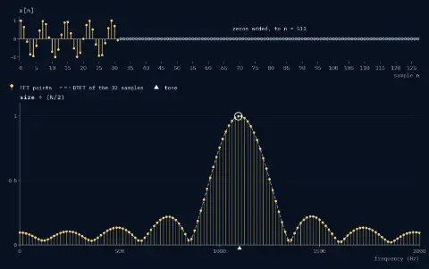
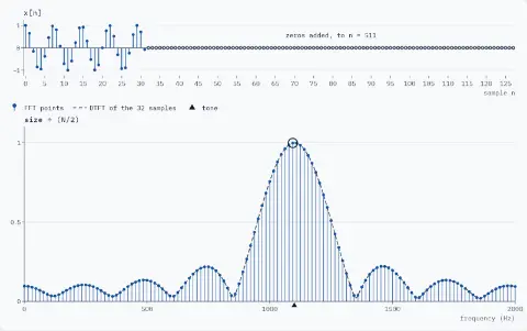
Top: the 32 samples of the tone as stems, then 480 zeros added, to n = 511. Bottom: size ÷ (N/2) against frequency from 0 to 2000 Hz. The DTFT of the 32 samples as a dashed curve, peaking at 1100.4 Hz with size 0.998; a triangle marks the tone at 1100 Hz. 512 FFT points, every 15.625 Hz, 129 of them from 0 to 2000 Hz, all on the curve; the highest, ringed, at 1093.75 Hz with size 0.997.Top: the 32 samples of the tone as stems, then 480 zeros added, to n = 511. Bottom: size ÷ (N/2) against frequency from 0 to 2000 Hz. The DTFT of the 32 samples as a dashed curve, peaking at 1100.4 Hz with size 0.998; a triangle marks the tone at 1100 Hz. 512 FFT points, every 15.625 Hz, 129 of them from 0 to 2000 Hz, all on the curve; the highest, ringed, at 1093.75 Hz with size 0.997.

Lesson 3 Essential20 minYou are hereRead

Zero-padding and resolution

Append zeros to a record and the FFT points come closer on the same curve. See why padding cannot split two tones, and how a parabola finds a peak between bins.

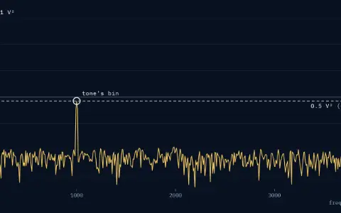
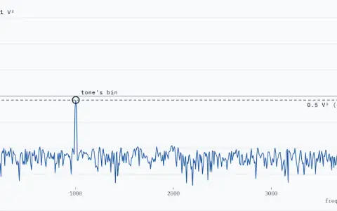
Spectrum of a 1 V, 1000 Hz tone plus noise, N = 1024, Hann window, against frequency from 0 to 4000 Hz, scaled as a² ÷ 2: power; vertical axis dB re 1 V² from −70 to 60. The tone's bin at 1000 Hz is ringed and reads −3.0 dB re 1 V². A dashed truth line at −3.0 dB is labelled 0.5 V² (−3.0 dB).Spectrum of a 1 V, 1000 Hz tone plus noise, N = 1024, Hann window, against frequency from 0 to 4000 Hz, scaled as a² ÷ 2: power; vertical axis dB re 1 V² from −70 to 60. The tone's bin at 1000 Hz is ringed and reads −3.0 dB re 1 V². A dashed truth line at −3.0 dB is labelled 0.5 V² (−3.0 dB).

Lesson 4 Essential22 minYou are hereRead

Reading a spectrum: scaling and units

Turn raw FFT numbers into volts, volts squared or volts squared per hertz, and learn which one reads a tone true and which reads noise true.

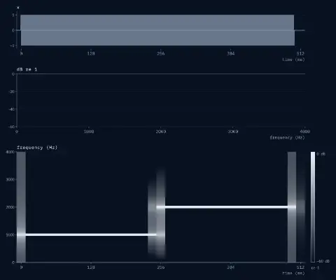
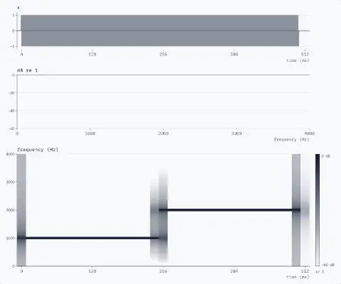
Signal sampled at 8 kHz: 1000 Hz for 0.25 s, then 2000 Hz, with its spectrogram below, frames of 256 samples every 16 ms. The spectrogram is complete: 33 columns, full ink at 1000 Hz up to 250 ms and at 2000 Hz after it.Signal sampled at 8 kHz: 1000 Hz for 0.25 s, then 2000 Hz, with its spectrogram below, frames of 256 samples every 16 ms. The spectrogram is complete: 33 columns, full ink at 1000 Hz up to 250 ms and at 2000 Hz after it.

Lesson 5 Essential19 minYou are hereRead

Spectrograms & the STFT

Cut a recording into windowed frames, take an FFT of each, and read the picture: tones as lines, clicks as stripes, glides as slopes.

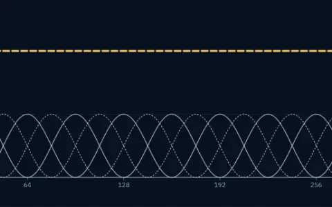
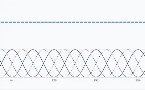
Hann windows of 64 samples, one every 16 samples (75 % overlap), drawn as thin lines on sample n from 0 to 320, neighbours alternating solid and dotted. Their sum, a thick dashed line, is flat at 2.000.Hann windows of 64 samples, one every 16 samples (75 % overlap), drawn as thin lines on sample n from 0 to 320, neighbours alternating solid and dotted. Their sum, a thick dashed line, is flat at 2.000.

Lesson 625 minYou are hereRead

Inverting the STFT

Add the frames of a spectrogram back to recover the sound, edit cells to erase or denoise it, and stretch time without changing pitch.

After this chapter

Where to go next.

The chapters either side, and the rest of Part V in the library.

Phasorium
LibraryEvery lesson, in order

Parts

About Phasorium
Look