Skip to content

Chapter 9

The Laplace transform

Three lessons in Part III, Fourier analysis of continuous-time signals. Read them in order, or start anywhere: a prerequisite is a link, never a gate.

Start with 9.1
0 of 3 read1 on the essential pathabout 85 minutes

Lessons in this chapter

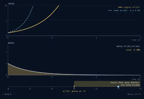
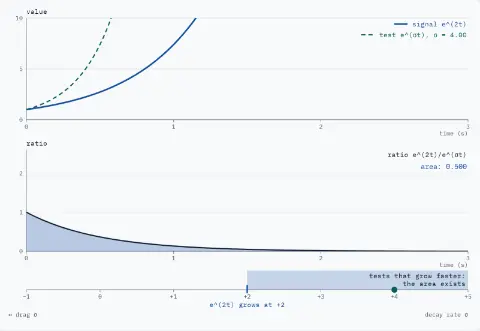
Top: the signal e^(2t), which grows at rate +2, and a test exponential e^(σt). Below: their ratio e^(2t)/e^(σt), with the area under it shaded. σ = 4.00. The ratio dies out. Readout: area: 0.500. Under the plot, the axis "decay rate σ" with a mark at +2, "e^(2t) grows at +2", and the region σ > 2 shaded: "tests that grow faster: the area exists".Top: the signal e^(2t), which grows at rate +2, and a test exponential e^(σt). Below: their ratio e^(2t)/e^(σt), with the area under it shaded. σ = 4.00. The ratio dies out. Readout: area: 0.500. Under the plot, the axis "decay rate σ" with a mark at +2, "e^(2t) grows at +2", and the region σ > 2 shaded: "tests that grow faster: the area exists".

Lesson 130 minYou are hereRead

The Laplace transform

Divide a signal by a test exponential, find which tests make the area exist, and read the Fourier transform off one line of the resulting plane.

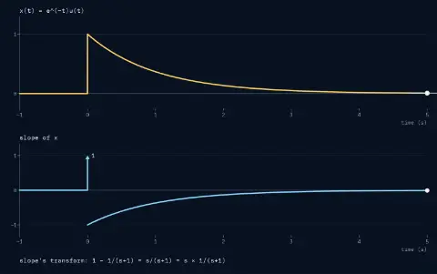
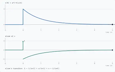
Top: x(t) = e^(−t)u(t), 0 before t = 0, jumping to 1 and decaying; a point rides it, now at t = 5.00 s, where x is 0.01 and the slope is −0.01. Bottom: the slope of x traced so far, with an arrow of area 1 at t = 0. The slope's transform so far: 1 − 1/(s+1) = s/(s+1) = s × 1/(s+1).Top: x(t) = e^(−t)u(t), 0 before t = 0, jumping to 1 and decaying; a point rides it, now at t = 5.00 s, where x is 0.01 and the slope is −0.01. Bottom: the slope of x traced so far, with an arrow of area 1 at t = 0. The slope's transform so far: 1 − 1/(s+1) = s/(s+1) = s × 1/(s+1).

Lesson 225 minYou are hereRead

Properties and the inverse Laplace transform

Turn differentiation into multiplication by s, split X(s) into one exponential per pole, and solve the charging capacitor again with algebra instead of calculus.

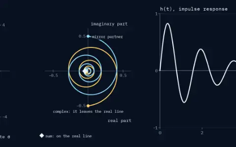
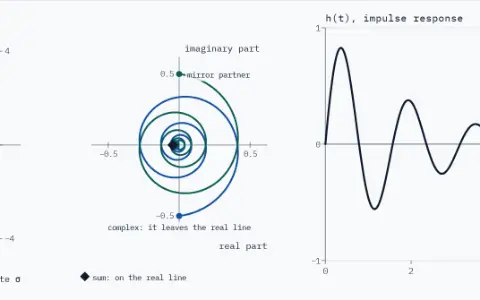
Plane of rates with the poles −0.5 + 4j and −0.5 − 4j. The panel of positions shows both spirals, and their sum on the real line tracing h(t) in the time panel.Plane of rates with the poles −0.5 + 4j and −0.5 − 4j. The panel of positions shows both spirals, and their sum on the real line tracing h(t) in the time panel.

Lesson 3 Essential30 minYou are hereRead

Poles, zeros and the s-plane

See why a real system's complex poles come in mirror pairs, how a pole's position sets the motion, and how feedback and zeros move or cancel poles.

Phasorium
LibraryEvery lesson, in order

Parts

About Phasorium
Look